In-Depth

Here are more careful details about why \(|\mathbb{R}^4| = |\mathbb{R}|\).

Rather than focus on \(|\mathbb{R}^4| = |\mathbb{R}|\), we will in fact show that \(|\mathbb{R}^n| = |\mathbb{R}|\) for any positive integer \(n\). As in the short explanation, we will prove the (notationally) simpler case of \(|\mathbb{R}^2| = |\mathbb{R}|\), and from the proof it will be clear how to do the case of general \(n\).

A key tool is the Cantor-Bernstein-Schroeder theorem. This theorem says that if an infinite set \(A\) can be put into one-to-one correspondence with a subset \(B\) of a set \(C\), then it makes sense to say \(| A| ≤ | C|\). And furthermore, if we can show \(| C| ≤ | A|\), then we can conclude that \(| A| = | C|\).

In other words, these sizes of infinities, which aren't really numbers, behave like numbers in this sense: \(a ≤ b\) and \(b ≤ a\) implies \(a = b\). We will use this theorem without proving it; the proof is surprisingly involved.

Our first step towards showing \(|\mathbb{R}^2| = |\mathbb{R}|\) will be to put \(\mathbb{R}\) into one-to-one correspondence with a subset of \(\mathbb{R}^2\). Remember that \(\mathbb{R}\) is the continuous one-dimensional real line, and \(\mathbb{R}^2\) is the continuous two-dimensional plane.

We can imagine a copy of \(\mathbb{R}\) sitting inside \(\mathbb{R}^2\), as the \(x\)-axis of a coordinate system. The elements of \(\mathbb{R}^2\) are of the form \([x, y]\), where \(x\) and \(y\) are real numbers. Then the \(x\)-axis is all the points of the form \([x, 0]\), where \(x\) is any real number. (The \(x\)-axis is exactly the points where the \(y\)-coordinate is zero.)

Figure: Coordinate axes drawn on a plane.

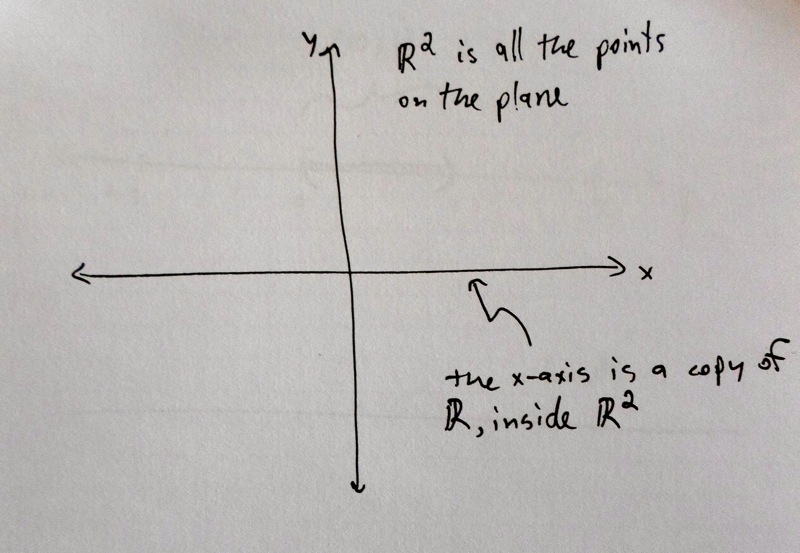
So we can construct a one-to-one correspondence between \(\mathbb{R}\) and the \(x\)-axis of the plane. Every real number \(x\) gets assigned to \([x, 0]\). This clearly hits every point on the \(x\)-axis once and only once. Since the \(x\)-axis is a subset of the whole plane \(\mathbb{R}^2\), we can use the Cantor-Bernstein-Schroeder theorem to conclude that \(|\mathbb{R}| ≤ |\mathbb{R}^2|\).

Next we will put \(\mathbb{R}^2\) into one-to-one correspondence with a subset of \(\mathbb{R}\). But here we have to be a little careful. Every element of \(\mathbb{R}^2\) can be written as \([x, y]\), but for many elements this is not unique. For example,

\[1 = 0.999999...\]

So the element \([1, 4]\) can be written as any of the following.

\[[1, 4]\\ [0.99999…, 4]\\ [1, 3.999999…]\\ [0.9999…, 3.9999…]\]

If we naively took each point \([x,y]\) and assigned it to the real number created by interweaving the digits of \(x\) and \(y\), as discussed in the short explanation, then we get into trouble. The same point \([1, 4]\) would get assigned to four different real numbers, depending on which representation we chose!

\[14\\ 04.9090909090…\\ 13.0909090909…\\ 03.9999999….\]

These are all very different real numbers.

To avoid this problem, we can declare which to choose. Let's choose the first. Now our assignment rule from \(\mathbb{R}^2\) to \(\mathbb{R}\) is: for each element \([x, y]\), write it in such a way that there are no endlessly-repeated nines. Then (after lining up the decimals and adding zeros to the left and right as necessary, so that both \(x\) and \(y\) have the same number of digits), interweave the digits of \(x\) and \(y\) to form one new real number.

Now this assignment rule is well-defined. And for every real number that gets hit by this assignment rule, it is possible to unweave the digits, to recover the element \([x, y]\) that hit it. In other words, this assignment rule makes a one-to-one correspondence between \(\mathbb{R}^2\) and the set of real numbers hit by the assignment rule.

But we still have one problem: not every real number gets hit by the assignment rule. For example, consider the real number

\[04.90909090…\]

If we unweave this real number, we get

\[[0.999999… , 4.00000].\]

But this is the same as \([1, 4]\), and according to our assignment rule this goes to \(14\). In other words, there is no element \([x,y]\) of \(\mathbb{R}^2\) that gets assigned to \(4.909090…\).

Fortunately this isn't a big problem. What we have shown is that there is a one-to-one correspondence between \(\mathbb{R}^2\) and a subset of \(\mathbb{R}\) (the subset of real numbers that do get hit by our assignment rule). Using the Cantor-Bernstein-Schroeder theorem we mentioned above, this is enough to conclude that \(|\mathbb{R}^2| ≤ |\mathbb{R}|\). And since we already showed that \(|\mathbb{R}| ≤ |\mathbb{R}^2|\), we have proved that \(|\mathbb{R}^2| = |\mathbb{R}|\).

To prove that \(|\mathbb{R}^4| = |\mathbb{R}|\), we would just have to alter the argument above to do a four-fold weaving. For example,

\[[1.01, 4.6, 0.8, 13]\]

would get assigned to

\[00011403.06801 = 11403.06801.\]

To prove that \(|\mathbb{R}^n| = |\mathbb{R}|\) for any positive integer \(n\), we would do an \(n\)-fold weaving.

Top